Introduction
NPL a super brief introduction
In this post we are going to have a look at what is called Natural Language Processing also known as NLP. First of all let’s define what is NLP. According to Wikipedia:
Natural language processing (NLP) is a subfield of linguistics, computer science, and artificial intelligence concerned with the interactions between computers and human language, in particular how to program computers to process and analyze large amounts of natural language data. The goal is a computer capable of “understanding” the contents of documents, including the contextual nuances of the language within them. The technology can then accurately extract information and insights contained in the documents as well as categorize and organize the documents themselves.
In brief NPL is a set of tools able to extract information from text data.
For this very introductory tutorial we will analyse the description of Netflix movies1 and trying to predict the film category using the description. In order to perform this task we will use above all those packages:
tidyversefor data manipulationtidymodelsfor modellingtidytextfor the analysis of text datatextrecipesfor additional text data recipes step
Importing the packages
library(tidyverse)
library(tidymodels)
library(tidytext)
library(textrecipes)
library(hrbrthemes)
theme_set(theme_light(base_size = 20))
Read data
The data is in .csv in order to read it we can use the readr::read_csv() function and save them in the netflix_titles variable.
netflix_titles <- readr::read_csv(path)## Rows: 7787 Columns: 12
## ── Column specification ────────────────────────────────────────────────────────
## Delimiter: ","
## chr (11): show_id, type, title, director, cast, country, date_added, rating,...
## dbl (1): release_year
##
## ℹ Use `spec()` to retrieve the full column specification for this data.
## ℹ Specify the column types or set `show_col_types = FALSE` to quiet this message.In order to have a look at the data we can use a very handy function from the dplyr which is glimpse().
dplyr::glimpse(netflix_titles)## Rows: 7,787
## Columns: 12
## $ show_id <chr> "s1", "s2", "s3", "s4", "s5", "s6", "s7", "s8", "s9", "s1…
## $ type <chr> "TV Show", "Movie", "Movie", "Movie", "Movie", "TV Show",…
## $ title <chr> "3%", "7:19", "23:59", "9", "21", "46", "122", "187", "70…
## $ director <chr> NA, "Jorge Michel Grau", "Gilbert Chan", "Shane Acker", "…
## $ cast <chr> "João Miguel, Bianca Comparato, Michel Gomes, Rodolfo Val…
## $ country <chr> "Brazil", "Mexico", "Singapore", "United States", "United…
## $ date_added <chr> "August 14, 2020", "December 23, 2016", "December 20, 201…
## $ release_year <dbl> 2020, 2016, 2011, 2009, 2008, 2016, 2019, 1997, 2019, 200…
## $ rating <chr> "TV-MA", "TV-MA", "R", "PG-13", "PG-13", "TV-MA", "TV-MA"…
## $ duration <chr> "4 Seasons", "93 min", "78 min", "80 min", "123 min", "1 …
## $ listed_in <chr> "International TV Shows, TV Dramas, TV Sci-Fi & Fantasy",…
## $ description <chr> "In a future where the elite inhabit an island paradise f…We can see that we have 7,787 rows and 12 columns. It seams also that the dataset contains also TV Shows. We can filter them out and select only the following columns:
titledescriptionlisted_in
Moreover using tidyr::separate_rows() we can split the word of the description column and create a table with a row for each word.
netflix_films <-
  netflix_titles %>%
  filter(tolower(type)  == "movie") %>%
  select(title, description, listed_in) %>%
  separate_rows(listed_in, sep = ", ")
Exploratory Data Analysis
Let’s first of all perform some Exploratory Data Analysis (EDA). A useful information could be counting the number of films by category. This can be done as follows:
netflix_films %>%
  count(listed_in, sort = T) %>%
  mutate(listed_in = fct_reorder(listed_in, n)) %>%
  ggplot(aes(x = n, y = listed_in, fill = n)) +
  geom_segment(aes(xend = 0, yend = listed_in),
    color = "grey50"
  ) +
  geom_point(aes(size = abs(n)),
    shape = 21,
    color = "grey50",
    show.legend = FALSE
  ) +
  scale_fill_viridis_c(option = "C") +
  scale_size_continuous(range = c(4, 7)) +
  labs(x = "Number of films", y = NULL)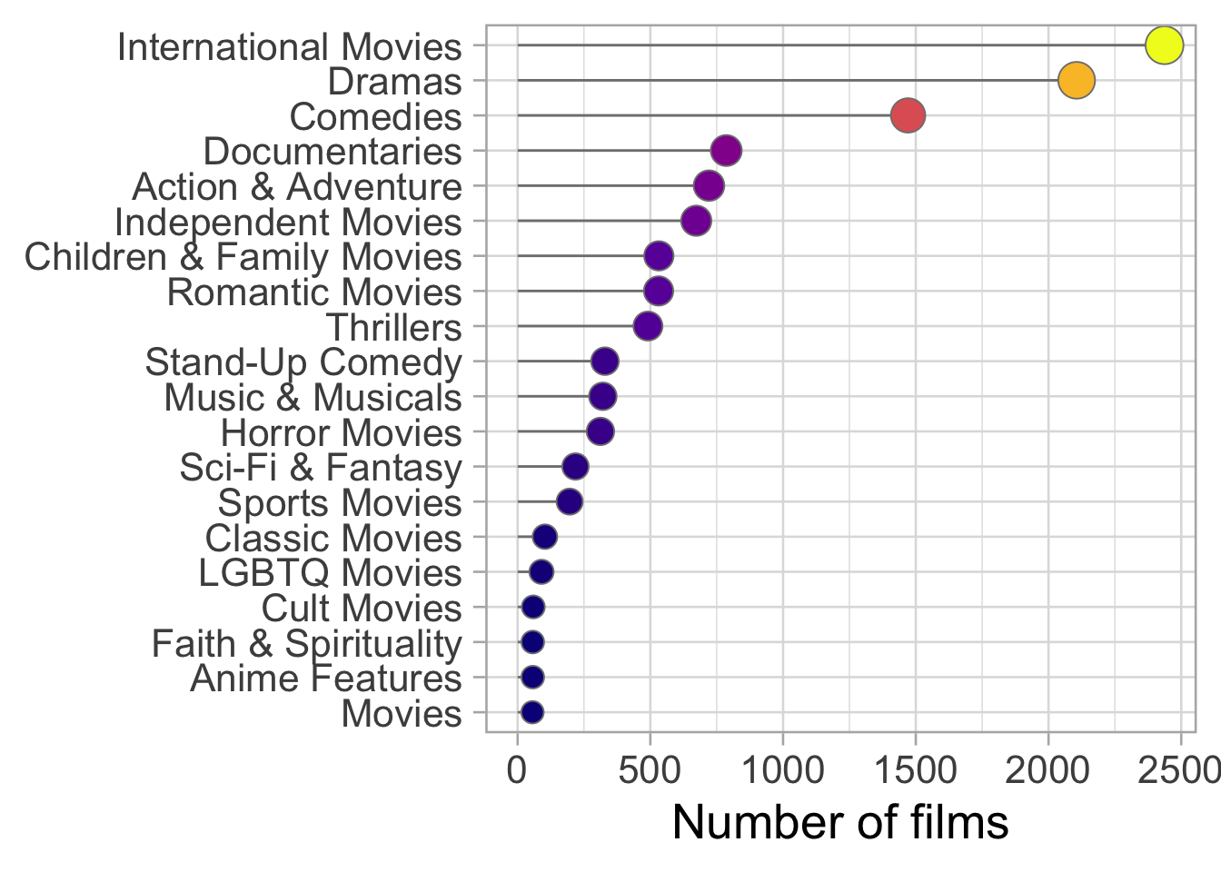
We have lots of categories!!!
Some of the categories have lots of observations, while other very few. This is not the optimal condition for a machine learning model.
We can follow different path here:
We can select some categories and collapse all the other into a macro category
We can select just few of them and drop all the others.
For the sake of this simple tutorial we will select just some categories which are:
Horror Movies
Children & Family Movies
Documentaries
In doing so we are left with 1,630.
category_to_select <-
    c("Horror Movies", "Children & Family Movies",
      "Documentaries")

netflix_films <- netflix_films %>%
  filter(listed_in %in% category_to_select)

netflix_films %>%
    count(listed_in, sort = TRUE) %>%
    knitr::kable(align = "lccrr",
caption = "Number of film by category")| listed_in | n |
|---|---|
| Documentaries | 786 |
| Children & Family Movies | 532 |
| Horror Movies | 312 |
As can be seen the number of observations for each category is a bit different. We can ask ourselfs whether the dataset is balanced or not. In order to answer this question we can use the Shannon Equitability Index which is a popular index to assess diversity. It is computed as follows:
\[ E_h=- \frac{\sum _{i=1}^{R}p_{i}\ln p_{i}}{\ln S} \]
where:
pi is the proportion of the samples belonging to the ith group
S is the total number of groups
shannon_index <- function(data_frame, class){
  result <- data_frame %>%
    count({{ class }}) %>%
    mutate(check =  - (n / sum(n) * log(n / sum(n))) /
             log(length({{ class }}))) %>%
    summarise(balance = sum(check))  %>%
    pull(balance)
    return(result)
}

netflix_films %>%
    count(listed_in) %>%
    mutate(sum_n = sum(n)) %>%
    mutate(check =  - (n / sum(n) * log(n / sum(n) ))) %>%
    summarise(balance = sum(check))
## # A tibble: 1 × 1
## balance
## <dbl>
## 1 1.03shannon_index_netflix <- netflix_films %>%
shannon_index(class = listed_in) %>%
round(digits = 2)
netflix_films %>%
mutate(film = "film") %>%
group_by(listed_in) %>%
add_count() %>%
ggplot(aes(film, fill = listed_in, label = n)) +
geom_bar(position = position_fill(), color = "black") +
scale_fill_ipsum() +
scale_y_percent(n.breaks = 8) +
labs(fill = NULL, x = NULL, y = "Percentage of film",
title = "Number of film per category",
subtitle = paste0(" Shannon Equitability Index: ",
shannon_index_netflix)) +
theme(legend.position = "bottom",
axis.ticks.y = element_blank(),
axis.text.y = element_blank(),
text = element_text(size = 18)) +
coord_flip() 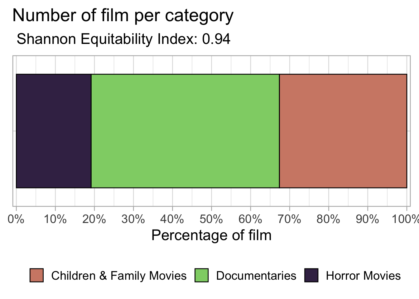
According to the Shannon Equitability Index the dataset is balanced. For this reason we can go on with our analysis.
We are now going to count the number of words by category. Ideally words that are recurrent in a category will be very useful in the modelling part.
As can be seen from the plot the most recurrent word in a category is documentary . As expected it is present a lot in documentary.
We can also notice that we have a problem with words like find and finds. This is a stemming problem but for the sake of this tutorial we will ignore this problem. If you are interested in what is stemming here the link to the Wikipedia page.
word_by_category <-
  netflix_films %>%
  unnest_tokens(word, description)  %>%
  anti_join(get_stopwords(), by = "word")  %>%
  count(word, listed_in,  sort = TRUE)   %>%
  group_by(listed_in) %>%
  slice_max(n = 15, order_by = n) %>%
  ungroup() %>%
  add_count(listed_in, name = "n_listed_in") %>%
  mutate(word = reorder_within(x = word, by = n,
                               within = listed_in))


ggplot(word_by_category, aes(n, word, fill = listed_in)) +
  geom_segment(aes(xend = 0, yend = word), color = "grey50") +
  geom_point(aes(size = abs(n)), shape = 21, color = "grey50",
             show.legend = FALSE) +
  facet_wrap(vars(listed_in), scales = "free_y", ncol = 1) +
  scale_y_reordered() +
  scale_fill_ipsum() +
  labs(y = NULL, x = "Number of word") +
  theme(text = element_text(size = 18)) +
  scale_size_continuous(range = c(3, 10))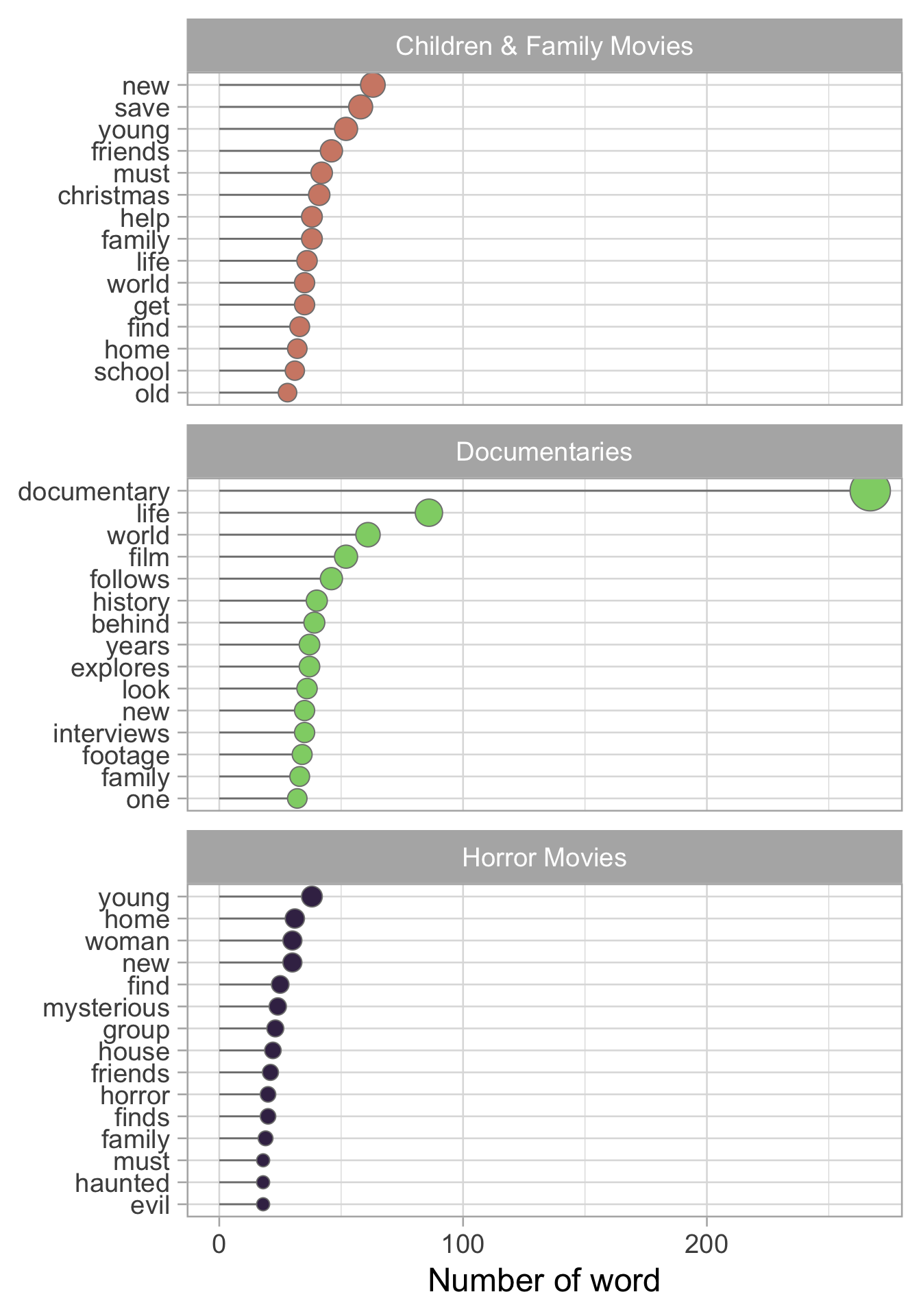
Unsupervised Analysis
Finally we can start to model our data. The first step is to split our data in training and testing set, in addition in we will create some resampling folds to perform the cross validation.
set.seed(123)
films_split <- initial_split(netflix_films, strata =  listed_in)

films_train <- training(films_split)
films_test <- testing(films_split)

set.seed(42)
films_folds <- vfold_cv(films_train, strata = listed_in)
From now on we will only work on the training films_train and films_testwill be used just to assess the quality of our model on new data at the end on the analysis.
A first type of analysis that we can make is performing a Principal Component Analysis. PCA is an unsupervised modelling analysis in which the original space generated by the predictors is transformed into another space in which the variance is maximized along the axis. On top of this PCA has another very interesting properties, the first PC is the one with the highest explained variance, the second PC is the second with the highest explained variance and so on.
But, in order to use PCA we have to transform the word in a numerical matrix. A very effective way to do that is using tf-idf.
In a very simple way tf e idf. The \(tf\) part is defined as follow:
\[ {tf_{i,j}} ={\frac {n_{i,j}}{|d_{j}|}} \]
\(n_{i,j}\) is the number of occurrence of the term \(i\) in the document \(j\)
\(|d_{j}|\) is the dimension of the document expressed in number of terms
While the \(idf\) parte is comuted as follow:
\[{idf_{i}} =\log _{10}{\frac {|D|}{|\{d:i\in d\}|}}\]
\(|D|\) is the number of document in the collection
\(|d_{j}|\) is the number of the document that contains the \(i\) document
In the end \(tf-idf\) is computed as:
\[ \mathrm {(tf{\mbox{-}}idf)_{i,j}} =\mathrm {tf_{i,j}} \times \mathrm {idf_{i}} . \]
As can be seen this matrix is very sparse and this is typical of text data.
films_rep_pca <-
  recipe(listed_in ~ description, films_train) %>%
  step_tokenize(description, options = list(lowercase = TRUE)) %>%
  step_stopwords(all_predictors()) %>%
  step_tokenfilter(all_predictors()) %>%
  step_tfidf(all_predictors())  %>%
  step_normalize(all_numeric_predictors())  %>%
  step_pca(all_numeric_predictors(), num_comp = 10)


films_juice_pca <-
  films_rep_pca %>%
  prep() %>%
  juice()
Looking at the PCA we can see that the first component divides quite well the Documentary and the Children & Family Movies while the second component divides Horror movies from the other two category.
p <- films_juice_pca %>%
  ggplot(aes(PC01, PC02, fill = listed_in)) +
  geom_point(shape = 21, size = 8) +
  scale_fill_ipsum(guide =
                       guide_legend(title = NULL,
                                    override.aes =
                                        list(size = 10))) +
  labs(x = "Principal component 1 (PC01)",
       y = "Principal component 2 (PC02)") +
  theme(legend.position = "top",
        text = element_text(size = 15))
plotly::ggplotly(p)
films_juice_pca %>%
pivot_longer(PC01:PC02) %>%
mutate(name =
if_else(name == "PC01",
"Principal component 1\n(PC01)",
"Principal component 2\n(PC02)")) %>%
ggplot(aes(name, value)) +
geom_violin(aes(fill = listed_in),
position = position_dodge(0.8), alpha = 0.8) +
geom_boxplot(aes(color = listed_in), show.legend = FALSE,
position = position_dodge(0.8), width = 0.1) +
scale_fill_ipsum() +
labs(fill = NULL, x = NULL, y = NULL) +
theme(legend.position = "top") +
scale_color_manual(values = rep("black", 3))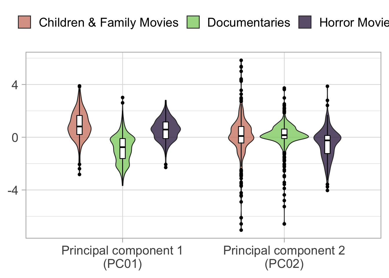
From the PCA we can obtain other information. Each principal component is a linear combination of the original columns. We can extract for each PC the word by which it is created by looking at the loading.
pca_loading <-
  tidy(films_rep_pca %>% prep(), number = 6, type = "coef") %>%
  filter(component %in% paste0("PC", 1:2)) %>%
  mutate(terms = str_remove(terms, "tfidf_description_"))  %>%
  mutate(sign = if_else(value > 0, "Positive", "Negative"))

pca_loading %>%
  mutate(label = if_else(abs(value) > 0.25,
                         round(value, 1), NULL)) %>%
  group_by(component) %>%
  slice_max(n = 25, order_by = abs(value)) %>%
  mutate(terms = reorder_within(terms, value, component)) %>%
  ggplot(aes(x = value, y = terms, fill = sign)) +
  geom_segment(aes(xend = 0, yend = terms), color = "grey50") +
  geom_point(aes(size = abs(value)), shape = 21,
             color = "grey50", show.legend = FALSE) +
  geom_text(aes(label = label), size = 2.5) +
  facet_wrap(vars(component), scales = "free_y", ncol = 1) +
  scale_fill_manual(values = c("#de2d26", "#31a354")) +
  labs(x = "Loading", y = NULL,
       title = "Top 25 word by component") +
  scale_size_continuous(range = c(2, 10)) +
  scale_y_reordered()  +
  theme(text = element_text(size = 15))
## Warning: Removed 45 rows containing missing values (geom_text).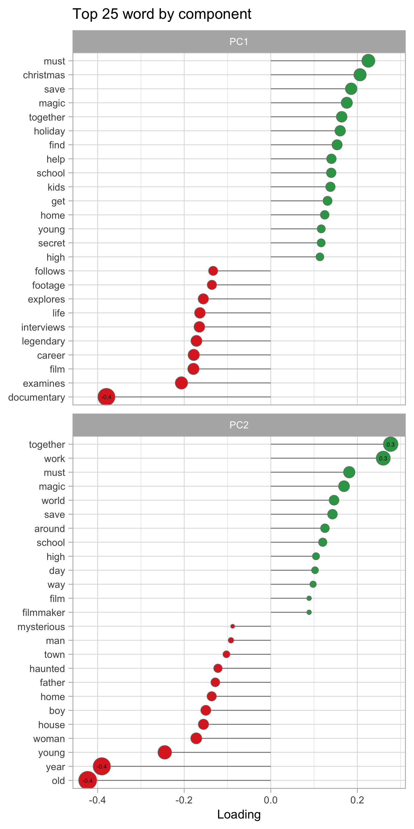
Modelling
Using the recipes a simple preprocessing recipe can be created. Then a model in this case a we are using linear support vector machine which works very well with text is created.
films_rep <-
  recipe(listed_in ~ ., films_train) %>%
  update_role(title, new_role = "ID") %>%
  step_tokenize(description, options = list(lowercase = TRUE)) %>%
  step_stopwords(all_predictors()) %>%
  step_tokenfilter(all_predictors()) %>%
  step_tfidf(all_predictors()) %>%
  step_normalize(all_predictors())

films_rep
## Recipe
##
## Inputs:
##
## role #variables
## ID 1
## outcome 1
## predictor 1
##
## Operations:
##
## Tokenization for description
## Stop word removal for all_predictors()
## Text filtering for all_predictors()
## Term frequency-inverse document frequency with all_predictors()
## Centering and scaling for all_predictors()svm_spec <- svm_linear(cost = 0.5) %>%
set_engine("kernlab") %>%
set_mode("classification")
svm_spec## Linear Support Vector Machine Model Specification (classification)
##
## Main Arguments:
## cost = 0.5
##
## Computational engine: kernlabIn order to train the model on our dataset we can take advantage of the tidymodel ecosystem and create a workflow object which can be seen as a place to store both preprocessing step and a model.
films_wf <- workflow() %>%
  add_recipe(films_rep)
films_wf
## ══ Workflow ════════════════════════════════════════════════════════════════════
## Preprocessor: Recipe
## Model: None
##
## ── Preprocessor ────────────────────────────────────────────────────────────────
## 5 Recipe Steps
##
## • step_tokenize()
## • step_stopwords()
## • step_tokenfilter()
## • step_tfidf()
## • step_normalize()doParallel::registerDoParallel(cores = 8)
set.seed(1234)
sv_film_res <- films_wf %>%
add_model(svm_spec) %>%
fit_resamples(
resamples = films_folds,
metrics = metric_set(roc_auc, accuracy, sens, spec),
control = control_grid(save_pred = TRUE, verbose = TRUE)
)The accuracy achieved by this simple model is \(68\%\) which is not extraordinary but is anyway good enough considering the little effort we have put. Moreover, if we create an empty model we obtain only an accuracy of \(48\%\) .
What is very good is that this model achieves a very high specificity which means that we have very low false positive. Which means that most of the time if for example it says “Documentary” it is actually a Documentary.
# NUll model

model_null <- null_model() %>%
  set_engine("parsnip") %>%
  set_mode("classification")

set.seed(1234)
workflow() %>%
    add_recipe(films_rep) %>%
    add_model(model_null) %>%
    fit_resamples(
        resamples = films_folds,
        metrics = metric_set(roc_auc, accuracy, sens, spec),
        control = control_grid(save_pred = TRUE, verbose = TRUE)
    )  %>%
    collect_metrics()
## # A tibble: 4 × 6
## .metric .estimator mean n std_err .config
## <chr> <chr> <dbl> <int> <dbl> <chr>
## 1 accuracy multiclass 0.482 10 0.000635 Preprocessor1_Model1
## 2 roc_auc hand_till 0.5 10 0 Preprocessor1_Model1
## 3 sens macro 0.333 10 0 Preprocessor1_Model1
## 4 spec macro 0.667 10 0 Preprocessor1_Model1sv_film_res_metrics <-
collect_metrics(sv_film_res) %>%
select(.metric, mean, std_err) %>%
mutate(.metric = case_when(
.metric == "roc_auc" ~ "roc auc",
.metric == "sens" ~ "sensitivity",
.metric == "spec" ~ "specificity",
TRUE ~ .metric))
sv_film_res_metrics %>%
ggplot(aes(.metric, mean, fill = .metric)) +
geom_errorbar(aes(ymin = mean - std_err,
ymax = mean + std_err),
width=.2, size = 2) +
geom_point(shape = 21, show.legend = FALSE,
size = 10) +
scale_y_continuous(labels =
paste0(seq(0.5, 1, 0.015) * 100, "%"),
breaks = seq(0.5, 1, 0.015)) +
labs(y = "10 folds cross validated value", x = NULL) +
scale_fill_manual(values = c("#f9b4ab", "#264e70",
"#679186", "#fdebd3"))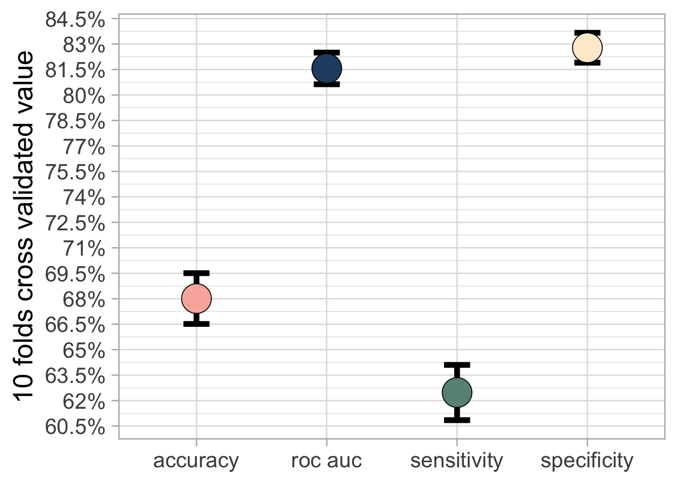
Using the vip package we can compute what are the features that influence the most our prediction. As we could expect documentary is the most important word but other word seems to be very useful in the classification. Examples are:
evil
Christmas
magic
library(vip)##
## Attaching package: 'vip'## The following object is masked from 'package:utils':
##
## vifilms_train %>% mutate(listed_in = factor(listed_in)) ## # A tibble: 1,222 × 3
## title description liste…¹
## <chr> <chr> <fct>
## 1 A Babysitter's Guide to Monster Hunting Recruited by a secret societ… Childr…
## 2 A Champion Heart When a grieving teen must wo… Childr…
## 3 A Christmas Prince Christmas comes early for an… Childr…
## 4 A Christmas Prince: The Royal Baby Christmas brings the ultimat… Childr…
## 5 A Christmas Prince: The Royal Wedding A year after helping Richard… Childr…
## 6 A Cinderella Story Teen Sam meets the boy of he… Childr…
## 7 A Fairly Odd Summer In this live-action adventur… Childr…
## 8 A Go! Go! Cory Carson Christmas When a familiar-looking stra… Childr…
## 9 A Go! Go! Cory Carson Halloween Cory, Chrissy and Freddie ar… Childr…
## 10 A Go! Go! Cory Carson Summer Camp Cory's spending the summer a… Childr…
## # … with 1,212 more rows, and abbreviated variable name ¹listed_in
## # ℹ Use `print(n = ...)` to see more rowsfilms_train$listed_in %>% unique()## [1] "Children & Family Movies" "Documentaries"
## [3] "Horror Movies"films_train$listed_in <-
fct_relevel(films_train$listed_in ,
ref = "Children & Family Movies")
set.seed(345)
films_imp <- films_wf %>%
add_model(svm_spec) %>%
fit(films_train) %>%
extract_fit_parsnip() %>%
vi(
method = "permute", nsim = 10,
target = "listed_in", metric = "accuracy",
pred_wrapper = kernlab::predict,
train = juice(films_rep %>% prep())
)## Setting default kernel parametersfilms_imp %>%
slice_max(Importance, n = 25) %>%
mutate(
Variable = str_remove(Variable, "tfidf_description_"),
Variable = fct_reorder(Variable, Importance)
) %>%
ggplot(aes(Importance, Variable, color = Importance)) +
geom_errorbar(aes(xmin = Importance - StDev,
xmax = Importance + StDev),
alpha = 0.5, size = 1.3) +
geom_point(size = 3) +
theme(legend.position = "top") +
labs(y = NULL, color = "Feature importance") +
scale_color_viridis_c(option = "C") +
guides(color = guide_colourbar(barwidth = 20,
title.position = "top")) 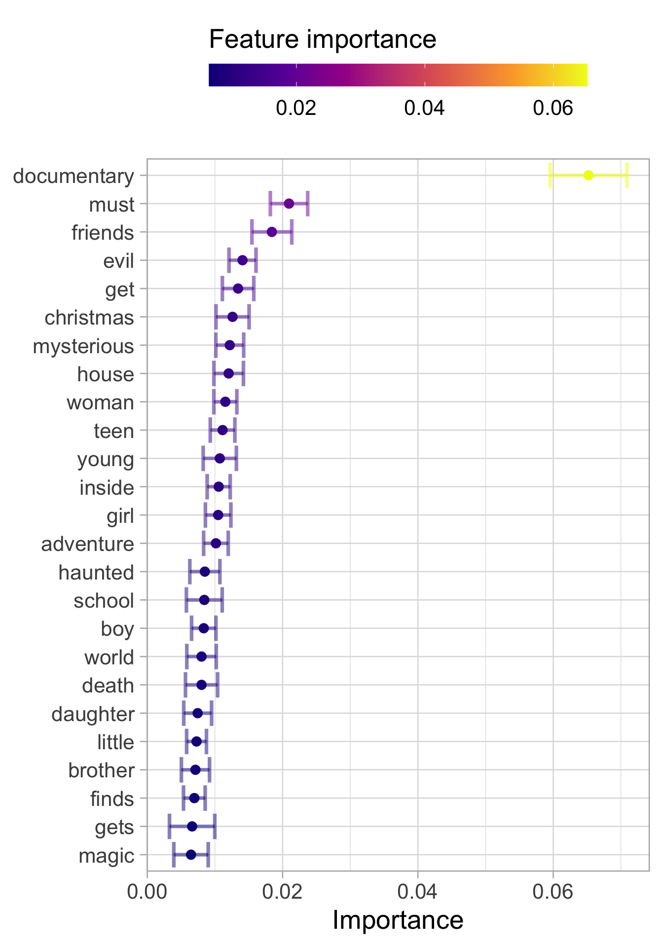
We can finally test out model on the test set and see if we overfitted or not.
films_final <- films_wf %>%
  add_model(svm_spec) %>%
  last_fit(films_split,
           metrics = metric_set(roc_auc, accuracy,
                                sens, spec))
Looking at the metrics and the confusion matrix it seams that we do not overfitted to much.
collect_metrics(films_final) %>%
  select(.metric, .estimate)  %>%
  mutate(.metric = case_when(
    .metric == "roc_auc" ~ "roc auc",
    .metric == "sens" ~ "sensitivity",
    .metric == "spec" ~ "specificity",
    TRUE ~ .metric
  )) %>%
    ggplot(aes(.metric, .estimate, fill = .metric)) +
    geom_segment(aes(xend = .metric, yend = 0.5),
               color = "grey50") +
    geom_point(shape = 21, show.legend = FALSE,
               size = 10)  +
    scale_y_continuous(labels = paste0(seq(0.5, 1, 0.015) *100,
                                     "%"),
                       breaks = seq(0.5, 1, 0.015)) +
    labs(y = NULL, x = NULL)  +
    scale_fill_manual(values = c("#f9b4ab", "#264e70",
                               "#679186", "#fdebd3"))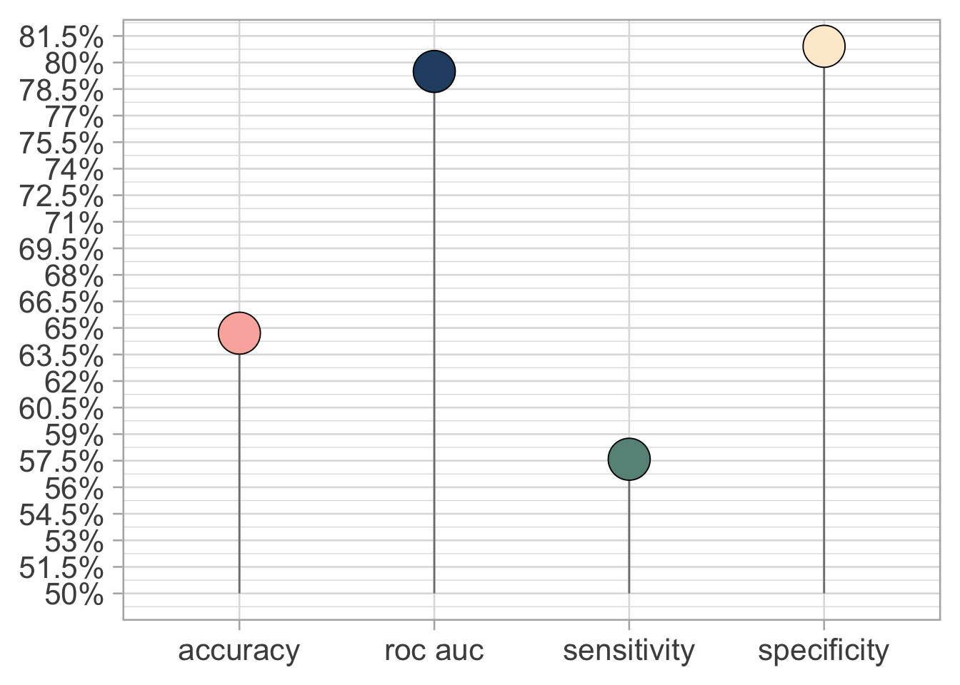
mat <- collect_predictions(films_final) %>%
  janitor::clean_names()   %>%
  conf_mat(pred_class, listed_in)

mat$table %>%
  data.frame()  %>%
  mutate(Prediction =
             str_replace(Prediction,
                         pattern = " & Family Movies",
                         "\n& Family \nMovies"),
         Truth =
             str_replace(Truth,
                         pattern = " & Family Movies",
                         "\n& Family \nMovies")) %>%

  ggplot(aes(Prediction, Truth, fill = Freq))  +
  geom_bin2d(bins = 100, color = "black") +
  geom_text(aes(label = Freq), size = 10) +
  scale_fill_continuous(type = "viridis")  +
  labs(x = "Predicted class", y = "True class",
       fill = "Frequency") +
  theme(legend.position = "top") +
  coord_fixed() +
  guides(fill = guide_colourbar(barwidth = 15),
text = element_text(size = 10)) 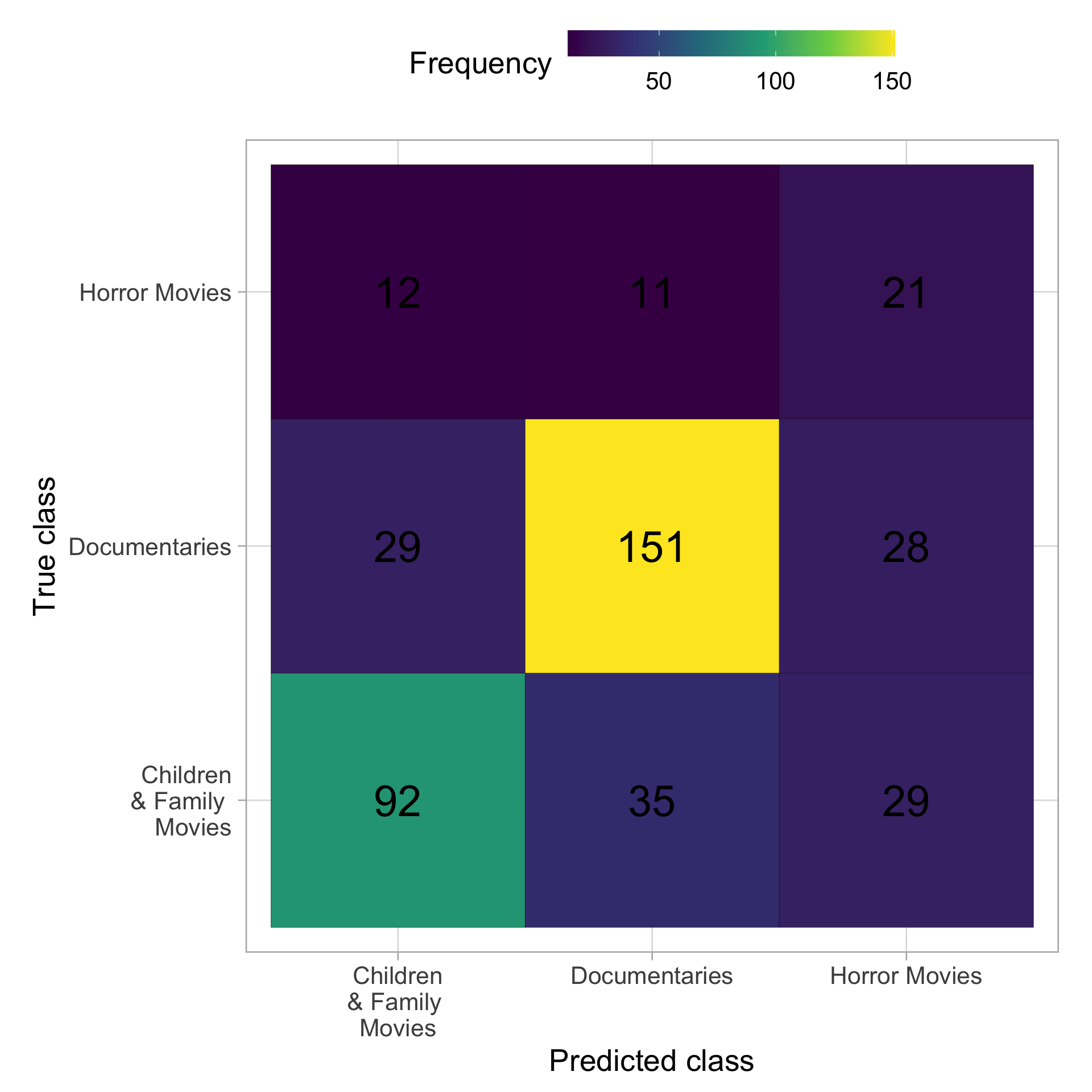
End
We have made through this analysis. In doing so, we have learnt that text data are very sparse, but linear models like PCA and linear SVM work very well with those type of data.
More information can be found here Netflix Shows↩︎