Import libraries

library("tidyverse")

Import data

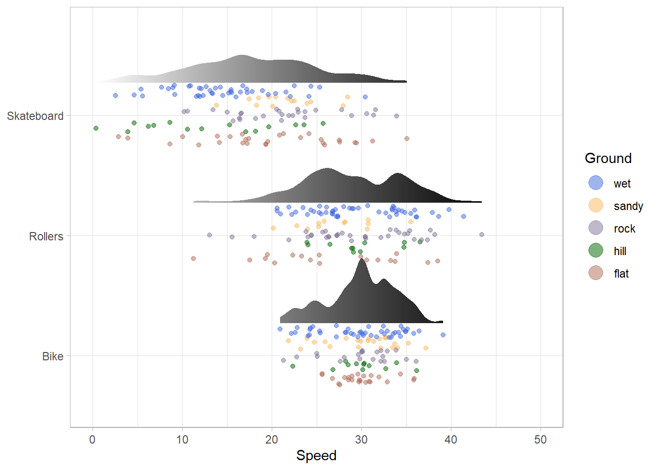
The dataset contains data about the speed of 3 different vehicles:

• bike
• skateboard
• rollers

Their speed is computed on 5 different grounds:

• sandy
• flat
• hill
• wet
• rock

The aim of the analysis is to observe the distribution of the speed of each vehicle to assess which one is faster.

frac<-readxl::read_excel("/Users/MariaRosariaNucera/Desktop/blog_data_science_bioinfo/Data/speed.xlsx")

Pivot dataframe

frac<-frac %>%
    pivot_longer(cols = c('Bike', 'Skateboard','Rollers'), 
                 names_to = "vehicle", 
                 values_to = "speed")%>%
    mutate(vehicle=fct_reorder(vehicle,speed))

Remove null values

frac<-na.omit(frac)

Plot

ggplot(frac, aes(x = vehicle, y = speed)) +
  geom_point(aes(colour = ground),
    position = position_jitterdodge(
      jitter.width = 0.1,
      dodge.width = 0.5
    ),
    alpha = 0.5
  ) +
  ggdist::stat_halfeye(aes(fill = stat(y)),
    adjust = .5,
    width = .6,
    show.legend = FALSE,
    .width = 0,
    justification = -.5,
    point_colour = NA
  ) +
  coord_flip() +
  ylim(0, 50) +
  labs(color = "Ground", x = NULL, y = "Speed") +
  scale_fill_gradient(low = "white", high = "black") +
  scale_colour_manual(
    values =
      c(
        "royalblue", "#FAB95B", "#827397", "darkgreen",
        "#AF6B58"
      ),
    limits = c("wet", "sandy", "rock", "hill", "flat")
  ) +
  theme_light() +
  guides(colour = guide_legend(override.aes = list(size = 5)))